
The Sequence of Price Delivery
From bullish expansion to Smart Money Reversal and bearish execution
Nasdaq Futures · October 5–9, 2026 · October 12 as subsequent review
The Sequence of Price Delivery
Reading the stages as they develop
This publication documents one week of Nasdaq futures price delivery, read stage by stage: bullish expansion, Smart Money Reversal, bearish execution. Its subject is how the founder interprets price as conditions develop. This research does not claim that the entire sequence was forecast in advance. It examines how contemporaneous structural observations anticipated specific stages of price delivery and how those observations evolved as market conditions developed.
Two distinctions organize the analysis.
Directional bias is not execution bias. Recognizing bullish conditions does not commit the analyst to buying indefinitely. Anticipating bearish opportunities does not authorize an immediate short. A Smart Money Reversal can mark the transition between stages of price delivery, and the analyst’s job is to identify the relevant stage and participate at an appropriate point in its delivery.
Predicting the eventual destination and identifying the appropriate entry are different analytical tasks. A higher-timeframe objective does not automatically authorize a position. Price may first need to trade higher — seek buy-side liquidity, establish a premium, complete a bullish leg within the relevant dealing range — before the conditions for a low-risk entry develop. Precision depends on understanding where price needs to go before the trade you actually want becomes available.
The operating frame is the founder’s own: ANALYST LEADS. TRADER OBEYS. RISK MANAGER DECIDES. The Analyst reads the stage of delivery. The Trader waits for executable conditions. The Risk Manager determines whether the proposed risk is acceptable.
Stage 1
October 5: Bullish Delivery
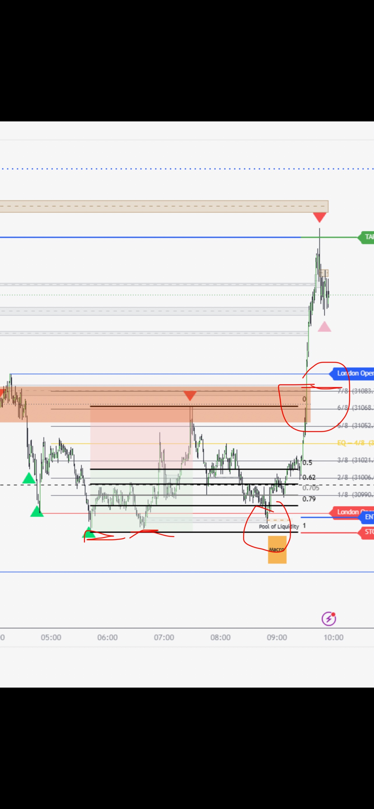
On Monday, October 5, the documented read was bullish. At 09:57, the founder wrote:
“Beautiful price delivery. 18.22R to buyside within internal dealing range highs. Entry during 0850 to 0910 macro inside of refined bullish fvg”
The recap describes a completed bullish delivery, not a forecast. The structure behind it was specific, and the founder laid it out in detail.
The dealing range
Price had been working inside a range within a range. The outer range ran roughly from 30,924.50 to 31,282.50, the latter being last week’s high. From Friday, October 2, price had sold off from the premium of that range all the way down to its discount. On Monday, the market offered a smaller range to work within, roughly 30,956.50 to 31,070.25. The trade lived inside the smaller range: entry 30,970.75, stop 30,957, target 31,221.25.
The objective
The target was buy-side liquidity. The founder was looking for session liquidity — the Asia session, between 20:00 and midnight, which had made a high. Whoever was short had stops above that high, so the founder was targeting it: “That’s an easy place to target.”
The timing
The entry came during the 8:50–9:10 macro window. In the founder’s framework, during specific price windows, price spools in a way that really displaces that time. During the macro, he watched every individual candlestick to confirm price was headed in the direction of the thesis — toward the buy-side liquidity of 31,221.25.
The entry location
The entry was inside a refined bullish PD Array, during the macro window. The stop sat at the low side of the smaller range — the point where the thesis would be wrong.
Read together, the elements form one analytical structure. The dealing range defines the territory. Session liquidity defines the objective. The macro window defines the timing. The PD Array defines the entry location. The stop defines invalidation. The founder was not buying merely because a bullish PD Array existed. He was evaluating it within a particular dealing range, during a particular time window, with a specific liquidity objective.
The founder was explicit about the directional read: “I’m not bearish. I’m bullish. The high timeframe is bullish.” That statement describes the stage as it stood on October 5. It is presented here in its original context.
Stage 2
October 7: Smart Money Reversal
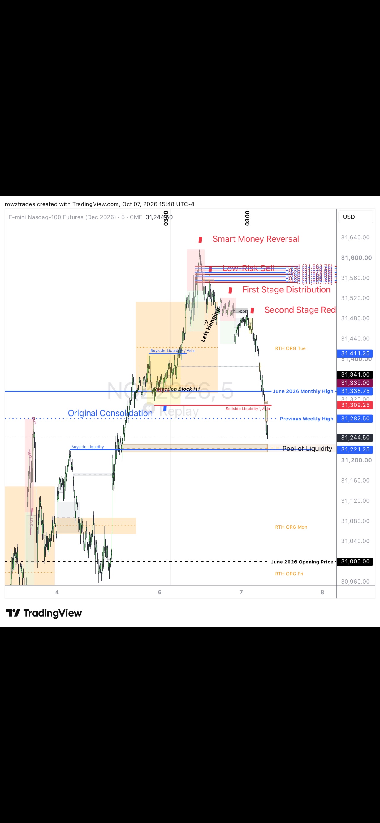
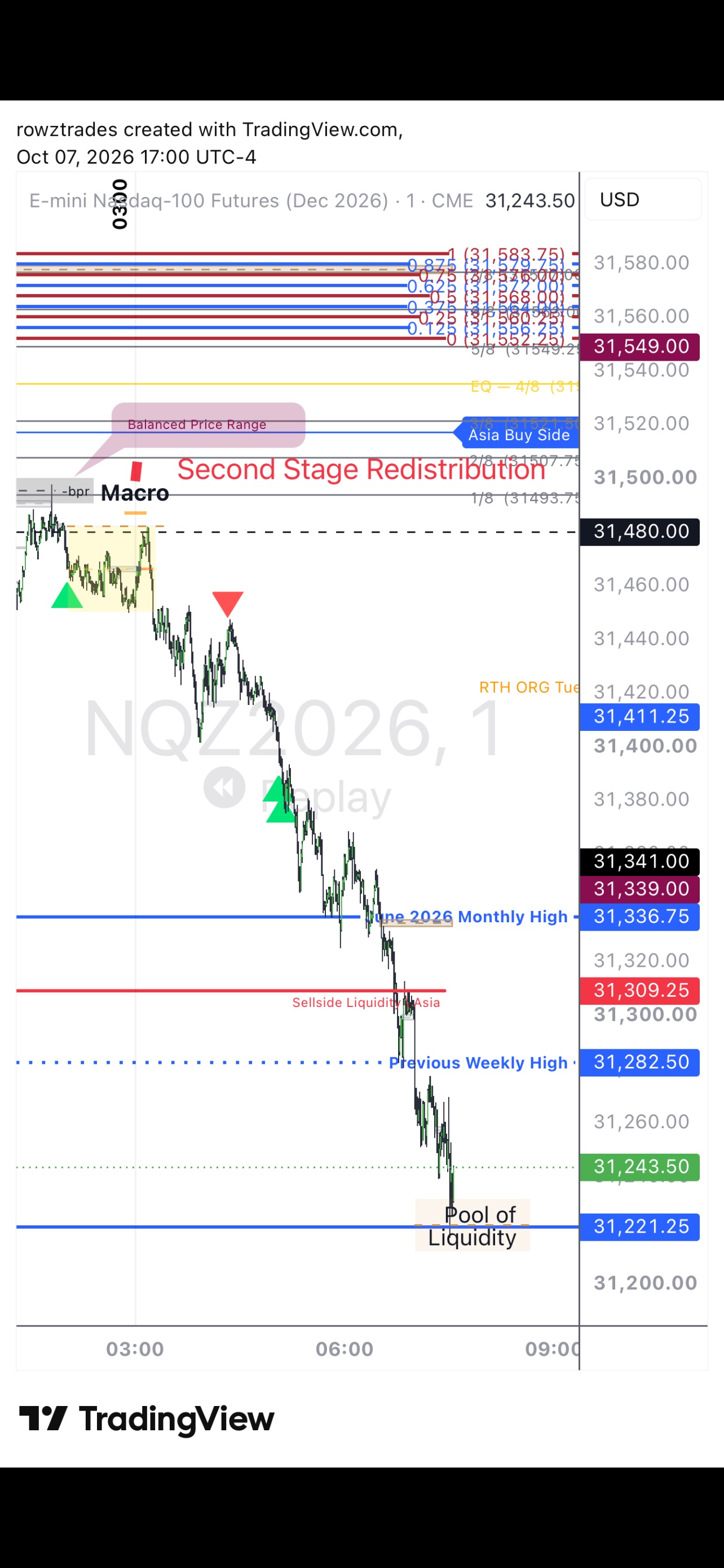
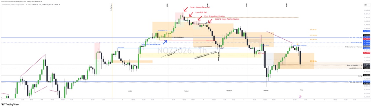
By October 7, the charts shared that day carried a different framework of annotations. Where the October 5 charts had described bullish delivery, the October 7 charts carried labels reading “Smart Money Reversal,” “Low-Risk Sell,” “First Stage Distribution,” “Second Stage Distribution,” and “Second Stage Redistribution.” The charts also carried the June 2026 Monthly High, the Previous Weekly High, and a Pool of Liquidity as reference levels. An October 6 chart already carried “Pool of Liquidity” and “Rejection Block H1.” The October 7 chart thumbnails also showed Asia Buy Side, Sellside Liquidity, Original Consolidation, Balanced Price Range, and Macro annotations.
The annotations are presented as evidence that the Smart Money Reversal and distribution framework appeared on charts shared that day. Their presence alone does not prove exactly when each annotation was originally created.
The annotations refer to the conventional ICT Market Maker Sell Model. That model identifies an initial consolidation, a buy-side advance, a Smart Money Reversal, and subsequent bearish distribution and redistribution. The Smart Money Reversal is the transition from the buy-side portion of the model toward bearish delivery. The Low-Risk Sell is the area associated with an opportunity to participate in the bearish movement. Distribution and redistribution are the subsequent stages of bearish delivery. The annotations organize observed price structure — short-term and intermediate-term swing highs and lows — into that model’s structure. They are labels applied to observed structure, not independent trading signals, and the publication attributes no predictive properties to the labels themselves. The Market Maker Model is ICT’s framework; the founder uses it within his broader Tesseract methodology to organize price delivery. The charts carry the monthly high, previous weekly high, and pool of liquidity as reference levels, and the October 7 chart thumbnails also carry an “Original Consolidation” annotation.
The October 7 message text, by contrast, was observational. At 17:20, the founder wrote:
“I love reading price action. So this is where price currently sits hrs after I sent the earlier screen shot. … Wicks do the damage. Bodies tell the story. … We know that we have a new dealing range from yesterdays high … and todays lows.”
The message records what the founder was watching: prior buy-side liquidity — the old high — holding the H1 bodies at bay. Wicks colored outside the lines, but that was acceptable: wicks do the damage, bodies tell the story. The H1 bodies stayed contained inside the overnight range — the box whose high was yesterday’s closing price and whose low was today’s opening price. Because the hourly bodies did not traverse further, the founder read a new dealing range, from yesterday’s high to today’s lows. He also noted that earlier screenshots had called the reversal, and that the sell-off to buy-side liquidity had been obvious.
No directional flip is stated in the October 7 messages. The charts show the reversal structure being read; the messages show the Analyst observing conditions — H1 candle bodies, the overnight range, a new dealing range.
Stage 2, continued
The Bearish Presentation
In subsequent messages appearing between the October 7 observations and October 9 execution, the founder discussed bearish SMT divergence and short participation. These messages are described by their position in the conversation. They carry no legible timestamps, and none is assigned.
The divergence
The founder compared ES, the correlated pair to NQ. Around 8, right before 9:00 — London Lunch, in the session-grading framework of eighths — ES went above its equilibrium while Nasdaq sold off from 9:30 to 10:00. That is divergence: what the founder marked with purple and pink carrots on the charts. He was explicit that these were not indicators:
“What those things are, it’s not indicators like a moving average or stochastics or what ICT calls Mickey Mouse horseshit. It’s literally objective things, like where the purple carrot is pointing down. Literally, ES made a higher high than NQ, or vice versa.”
The read that followed was about direction of travel: “I know that we need to go towards discount once I see that. That’s what I did: I went short there.”
The discount-side read
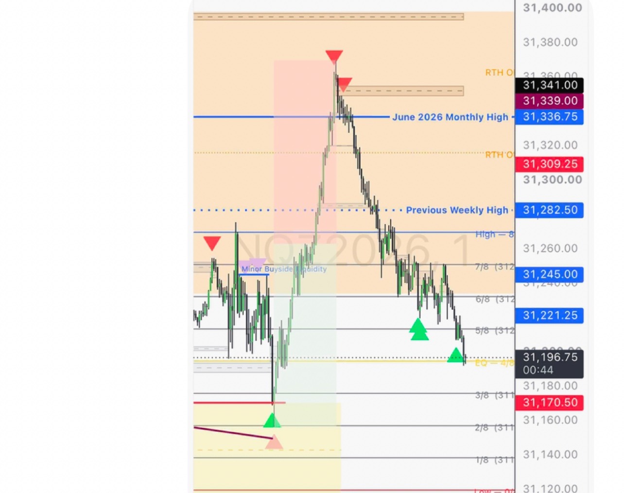
Price was back on the discount side of the range that had formed during regular trading hours. On the chart, price had revisited the June 2026 monthly high. The founder had SMT, as indicated by the red carrots:
“I had SMT, as indicated by the red carrots…”
The message also describes a refined range that price never revisited after it made the overlay. His conclusion was conditional:
“I would have been comfortable shorting the monthly high all the way back towards discount, at least equal to equilibrium of discount, and then holding a runner until I got a bullish carrot.”
The passage shows the full structure of the bearish presentation: the monthly high as the reference level, SMT as the confirming divergence, the discount side as the objective, equilibrium of discount as the minimum target, and a runner held until a bullish carrot — a bullish SMT signal — marked the exit. Three bullish carrots eventually appeared, and the founder noted he would also watch the initial range of price action that had sent price up in the first place.
Note the conditional phrasing: would have been comfortable. This is an articulation of reversal conditions, not a claim about a single continuous position.
Stage 3
October 9: Executing the Delivery
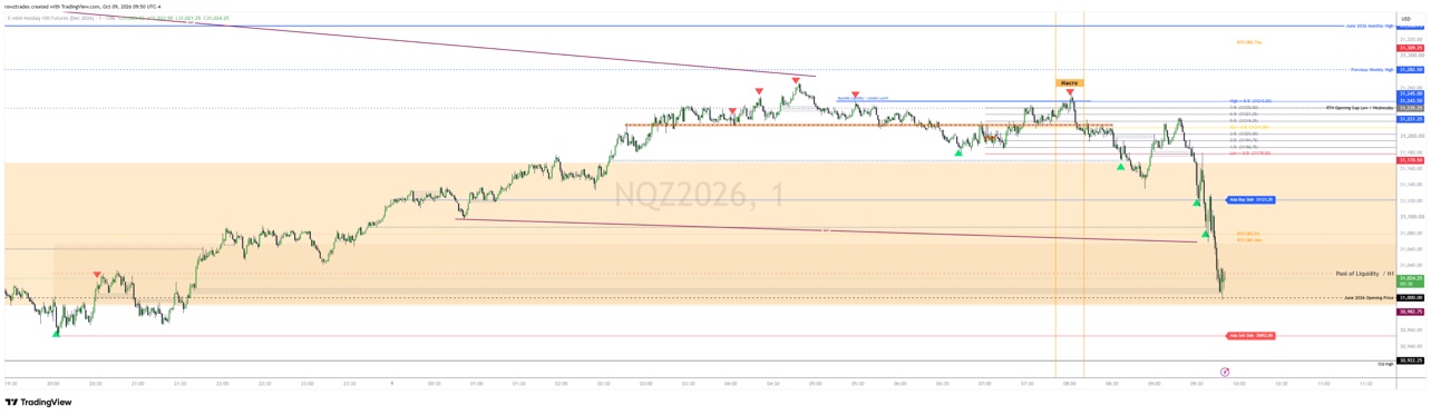
On Friday, October 9, the founder executed a short toward a higher-timeframe downside objective he had identified that morning:
“Was looking for H1 pool of liquidity CE from my analysis early this morning.”
The statement is the analytical core of the execution. The H1 pool of liquidity consequent encroachment was the downside objective — the level price was delivering toward — identified before the session. It was not the entry location.
The chart evidence fixes the objective zone. The October 9 1H chart labels a Pool of Liquidity / H1 at 31,041.75, with the June 2026 Opening Price at 31,000.00 below it. The founder’s figure for the H1 PD Array’s consequent encroachment, near 31,008.50, sits in that zone.
The trade itself was entered above the objective zone: entry 31,203, stop 31,253.50 (202 ticks) above the entry, targets 31,032.00 (684 ticks) and 31,011.50 (766 ticks) set as price approached the objective zone. The Discord execution record shows “Order Filled” on 10/9 at 09:45. Exits are documented via execution markers on the TradingView charts.
| Reference | NQ price | Analytical role |
|---|---|---|
| Short entry | 31,203.00 | Execution |
| Stop | 31,253.50 | Structural invalidation |
| H1 pool of liquidity | 31,041.75 | Downside objective zone |
| First target | 31,032.00 | Execution objective |
| Second target | 31,011.50 | Extended objective |
| June opening price | 31,000.00 | Additional higher-timeframe reference |
The relationship between the objective, the intraday structure, and the execution is the substance of this section. The H1 pool is a higher-timeframe reference — a zone where liquidity rests. The trade shorts from above that zone, with the stop above the entry marking the point where the thesis fails, and the targets set as price delivers into the objective zone. The trade is a short entered above a pre-identified downside objective, with defined invalidation.
This execution is a separately documented trading decision. It is not presented as the continuation of the short discussed in the subsequent messages.
Subsequent review
October 12: Reviewing the Sequence
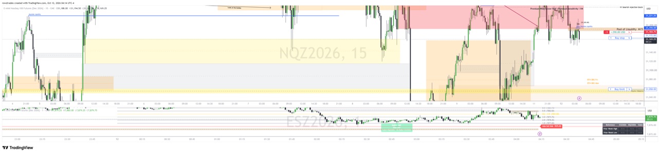
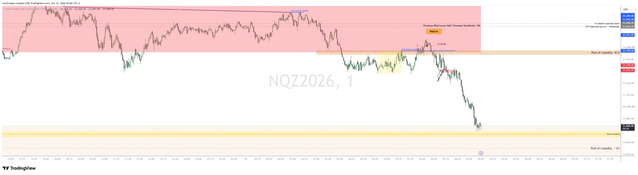
On Monday, October 12, at 05:10, the founder reviewed Friday’s London session:
“Easy call. Called the high at 0350 to the low at 0455. 144 handles from 31203 (consequent encroachment of premium wick to weekly volume imbalance) to 31059 (volume imbalance)…”
The review is a subsequent observation of Friday’s London delivery, presented as such. It is not part of the October 5–9 stages, and it is not treated as evidence for what was known during the week. Its analytical content is the labeling: 31,203 as the consequent encroachment of a premium wick to the weekly volume imbalance, and 31,059 as the volume imbalance itself — the levels that bounded the London move.
Analytical Synthesis
How the stages relate
This section is retrospective interpretation. It explains how the stages relate under the founder’s methodology. It is not a claim that the full sequence was identified in advance on October 5.
The October 5–9 record shows successive stages of price delivery:
Bullish delivery → Completion of an objective → Smart Money Reversal → Bearish delivery.
Each stage was documented as it developed. The bullish delivery of October 5 moved price toward buy-side liquidity. The October 7 charts show the reversal and distribution framework being read. The subsequent messages articulate the reversal conditions — SMT divergence, the monthly-high revisit, the discount-side objective. October 9 shows execution in bearish delivery toward a pre-identified H1 objective.
This is a coherent sequence reconstructed from contemporaneous observations. The publication explains the relationship among the stages.
Three points in the methodology explain why the stages cohere:
A bullish read at one stage does not contradict a bearish read at the next. The stages are successive, not competing. The founder was not bullish-then-wrong. He read each stage as it developed, and each stage’s read was appropriate to its conditions.
Destination versus entry. The entry was established independently of the higher-timeframe destination. The objective told the founder where price might deliver. The execution model determined whether and where he could participate. Price must first move to establish the conditions for a low-risk entry — seeking liquidity, establishing premium, completing the dealing-range objective. The bullish leg is not an obstacle to the bearish thesis; it can be the movement that creates the conditions for the reversal.
Anyone can recognize an SMT divergence. Anyone can recognize a PD Array. Anyone can identify a previous weekly high. But those observations do not independently establish whether an opportunity deserves participation. The analytical process seeks to understand the relationship between those formations — their location, their timing, and the stage of price delivery. A formation becomes relevant at a particular time, in a particular dealing range, after particular liquidity conditions have developed.
The formation alone is not the analysis. The sequence is.
That is the expertise this publication makes visible: not the ability to identify the next bullish or bearish move, but the ability to explain why a particular market movement matters within the larger sequence of price delivery.
Research Notes
Method & boundaries
- This publication distinguishes contemporaneous observations from subsequent interpretation. The Analytical Synthesis is retrospective; the stage sections report what was documented at the time.
- Some message timestamps are not independently established. Those messages are placed by their position in the conversation, and no timestamp is assigned where the record does not show one.
- Execution records are treated separately from analytical commentary. The October 9 execution is a separately documented trading decision.
- This study does not claim that the entire price-delivery sequence was anticipated on October 5.
- Quotations are the founder’s only, excerpted from his messages. The other participant in the thread is not quoted or identified.